Data Entry
Excel Tutorial
This tutorial is designed to assist the beginner and refresh the experienced Excel user on some of the skills that will be needed in the IAAO Mass Appraisal courses. Accompanying this tutorial is an Excel worksheet containing sample data for your use. Please save that file to another location on your computer, using a different name. This will avoid corrupting the original file.
Access the Excel worksheet here.
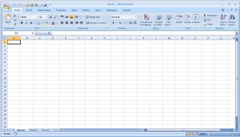
When you start Excel you're faced with a big empty grid. There are letters across the top and numbers down the left side. And there are tabs at the bottom named Sheet1, Sheet2, and Sheet 3.
If you're new to Excel, you may wonder what to do next.
We'll begin by helping you get comfortable with some Excel basics that will guide you when you enter data in Excel.
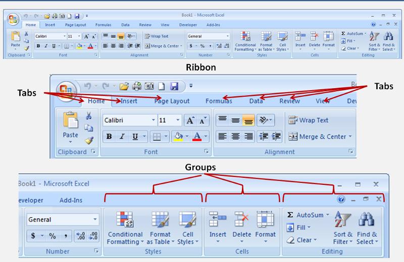
The band at the top of the Excel 2007 window is the Ribbon. The Ribbon is made up of different tabs. Each tab is related to specific kinds of work that people do in Excel. You click the tabs at the top of the Ribbon to see the different commands on each tab. The Home tab, the first tab on the left, contains the everyday commands that people use the most.
Commands are organized in small related groups. For example, commands to edit cells are grouped together in the Editing group, and commands to work with cells are in the Cells group.
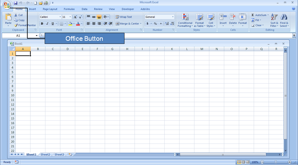
In the upper left corner of the workbook is the Office Button. It operates in much the same way as the File menu in older versions of Excel. You can access basic functions that are available in most programs, such as opening, saving and closing files.
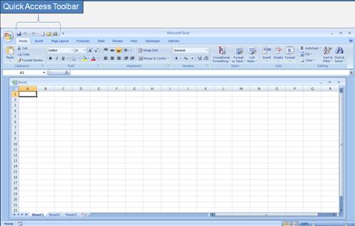
Those functions that are used most often can be placed at the top of the workbook in an area called the Quick Access Toolbar.
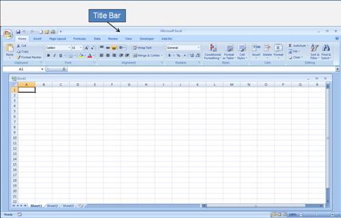
The Title Bar is found at the top center of the workbook and it will display either a default name such as Workbook 1 or the name under which the workbook was last saved. This is very helpful when you have several workbooks open.
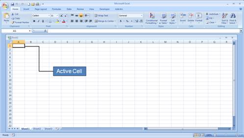
Notice that a single cell in the upper left corner of the worksheet is highlighted. This is called the Active Cell. It is the cell that can receive input. You, the user, select which cell that will be.
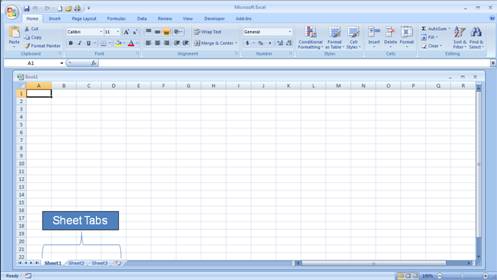
Sheet Tabs are initially named Sheet 1, Sheet2 and Sheet 3. It's a good idea to rename the sheet tabs to make the information on each sheet easier to identify. This is done by right clicking on them and selecting the option rename from the pop-up menu. Additional sheets can be added to the workbook by clicking on the far right tab that is not named. And you can use keyboard shortcuts to move between sheets.
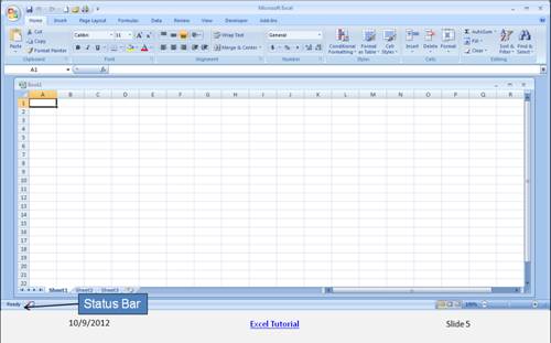
The Status Bar in the lower left corner tracks the actions of the user. For example, the status of the worksheet in our slide shows it is Ready to receive data. When the user starts entering data, the status will change to Enter.

The Sheet Tab Scroll Buttons are another means of navigating between sheets of the workbook other than selecting a tab. The value of this functionality will become more evident with the use of multiple worksheets.
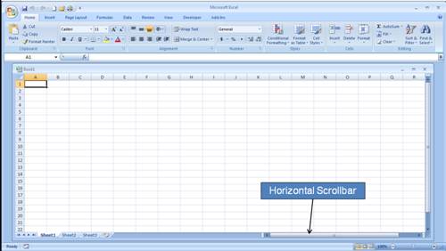
As more data is entered across the worksheet, the user will find the Horizontal Scrollbar useful for moving around the worksheet and locating a particular cell.
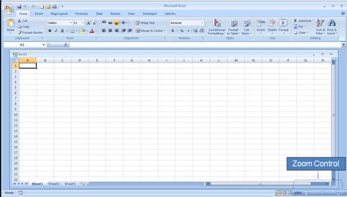
The Zoom Control is another means of locating and focusing attention on a particular part of the active worksheet.
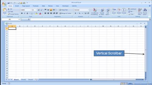
Finally, the Vertical Scrollbar provides yet another means of maneuvering around the active worksheet.
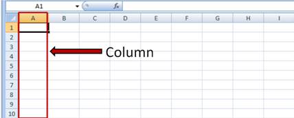
Worksheets are divided into columns, rows, and cells. That's the grid you see when you open up a workbook.
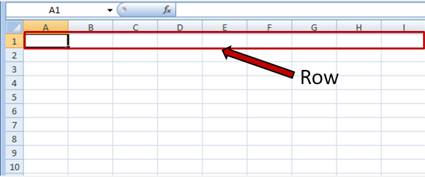
Columns go from top to bottom of the worksheet, vertically. Rows go from left to right on the worksheet, horizontally. A cell is the space where one column and one row meet.
Each column has an alphabetical heading at the top. The first 26 columns have the letters from A through Z. Each worksheet contains 16,384 columns in all, so after Z the letters begin again in pairs, AA through AZ.
After AZ, the letter pairs start again with columns BA through BZ, and so on, until all 16,384 columns have alphabetical headings.
Each row also has a heading. Row headings are numbers, from 1 through 1,048,576.
The alphabetical headings on the columns and the numerical headings on the rows tell you where you are in a worksheet when you click a cell. The headings combine to form the cell address, also called the cell reference.
Cells are where you get down to business and enter data in a worksheet.
When you open a new workbook, the first cell you see in the upper-left corner of the worksheet is outlined in black, indicating that any data you enter will go there.
You can enter data wherever you like by clicking any cell in the worksheet to select the cell. But the first cell (or one nearby) is not a bad place to start entering data in most cases.
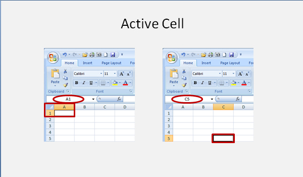
When you select any cell, it becomes the active cell. When a cell is active, it is outlined in black, and the headings for the column and the row in which the cell is located are highlighted.
For example, if you select a cell in column C on row 5, the headings on column C and row 5 are highlighted, and the cell is outlined. That cell is known as cell C5, which is the cell reference.

The outlined cell and the highlighted column and row headings make it easier for you to see that cell C5 is the active cell. Also, the cell reference of the active cell appears in the Name Box in the upper-left corner of the worksheet. By looking in the Name Box, you can see the cell reference of the active cell.
All of these indicators are not too important when you're right at the very top of the worksheet in the very first few cells. But when you work further and further down or across the worksheet, they can really help you out. Keep in mind that there are 17,179,869,184 cells to work in on each worksheet. You could get lost without the cell reference to tell you where you are.
For example, it's important to know the cell reference if you need to tell someone where specific data is located or must be entered in a worksheet.
You can enter three basic kinds of data into worksheet cells: numbers, text and dates.
In the Mass Appraisal courses, you will be using real estate data supplied to you. However, it is important for you to know how to enter and manipulate data in a worksheet. The worksheet used to create this tutorial represents actual sales data.
When you enter or import data into a worksheet, it's a good idea to enter titles at the top of each column so that anyone who shares your worksheet can understand what the data means (and so that you can understand it yourself, when you come back to it).
In the picture on the next page, the column titles are the names of data fields from a CAMA system. Each of the rows represents an individual parcel record.
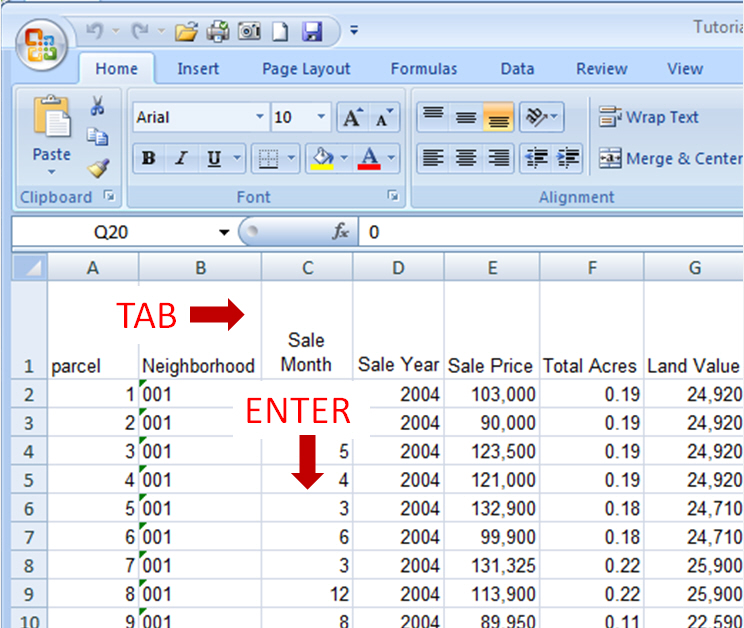
There are several ways of moving around a worksheet. As you enter titles across the top, press the TAB key to move from one column to the next or from one field to the next.
Once you are in a field, you can enter information for several records by striking the ENTER key after each entry.
The arrow keys can be used, but may not be as easy to use as the TAB and ENTER keys.
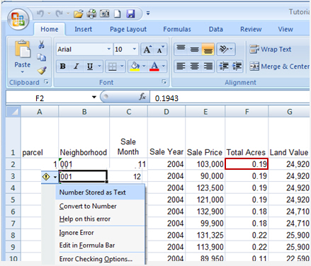
It is important to understand how Excel treats certain data. For example, text fields will accept data exactly as entered, whereas numeric fields will drop leading zeros and extraneous decimal places. Column B in the above worksheet is a text field in which the user has entered numbers with leading zeros. The zeros are retained. If column B were a numeric field, the zeros would be dropped. Note the small triangles in the cells in column B. When the user clicks on any of the cells in that column, a symbol appears to the left of the cell ![]() .
.
Clicking on that symbol causes a menu of possibilities to pop up. In this case, the cell contains a number stored as text. The neighborhood identifier is "001". It is entered as text to retain the leading zeros. Otherwise, the cell would contain just 1.
In Excel what you see is not always what you get. Cell F2 appears to contain the data 0.19. However, that is just the way the data has been formatted. In reality, the cell contains 0.1943 that has been rounded to 0.19 for purposes of display only. Excel will use the underlying data of 0.1943 in calculations, which may produce unexpected results (24,920 / .1943 = 128,255 instead of 24,920 / .19 = 131,158).
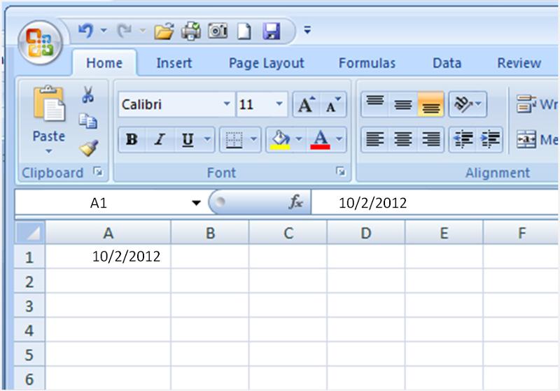
To enter a date, you should use a slash or a hyphen to separate the parts: 7/16/2009 or 16-July-2009. Excel will recognize this as a date.
If you need to enter a time, type the numbers, a space, and then "a" or "p" — for example, 9:00 p. If you put in just the number, Excel recognizes a time and enters it as AM.
Tip To enter today's date, press CTRL and the semicolon (;) together. To enter the current time, press CTRL and SHIFT and the semicolon all at once.
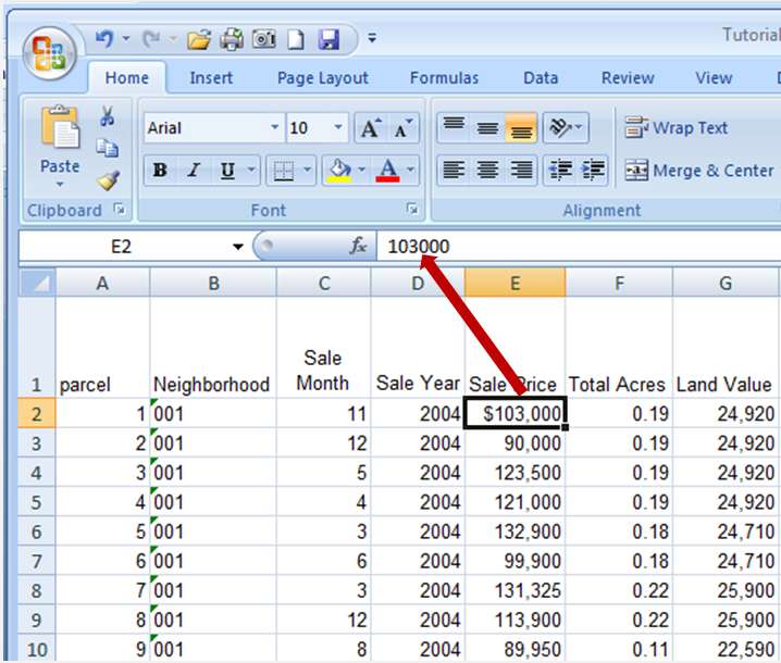
This slide illustrates another difference between display and underlying data. The sale price at E2 is displayed as $103,000 while the underlying data is 103000.
Other numbers and how to enter them
Here are two time-savers you can use to enter data in Excel:
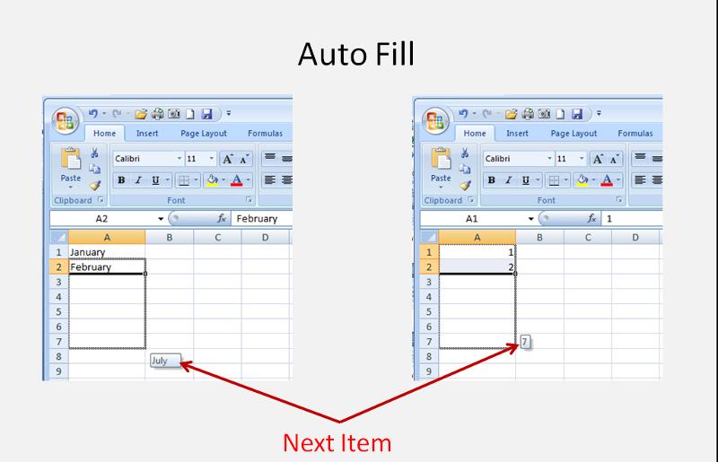
AutoFill Enter the months of the year, the days of the week, multiples of 2 or 3, or other data in a series. You type one or more entries, and then extend the series by dragging. Notice the next item in the series appears next to the bottom right corner of the dragged section. Once the dragging stops, the cells are filled with the next items in the series.
AutoComplete If the first few letters you type in a cell match an entry you've already made in that column, Excel will fill in the remaining characters for you. Just press ENTER when you see them added. This works for text or for text with numbers. It does not work for numbers only, for dates, or for times.
Everyone makes mistakes sometimes, and sometimes data that you entered correctly needs to be changed later on.
Sometimes the whole worksheet needs a change. Suppose you need to add another column of data, right in the middle of your worksheet.

Say that you meant to enter 125,000 in cell E4, but you entered 123,500 by mistake. Now you spot the error and want to correct it. There are two ways to do it:
What's the difference? Your convenience. You may find the formula bar, or the cell itself, easier to work with. If you are editing data in many cells, you can keep your pointer at the formula bar while you move from cell to cell by using the keyboard.
After you select the cell, the worksheet says Edit in the lower-left corner, on the status bar.
While the worksheet is in Edit mode, many commands are temporarily unavailable (these commands are gray on the ribbon).
What can you do? Well, you can delete letters or numbers by pressing BACKSPACE, or by highlighting (selecting) them and then pressing DELETE.
You can edit letters or numbers by highlighting (selecting) them and then typing something different.
You can insert new letters or numbers into the cell's data by positioning the cursor at an insertion point and typing.
Whatever you do, when you're all through, remember to press ENTER or TAB so that your changes stay in the cell.

Surprise! Someone else has used your worksheet, filled in some data, and made the number in cell E4 bold, red and $133,000.
But you know the actual selling price was $123,500. You delete the original figure and type in the new number.
But the new number is still a bold red number. What gives here?
What's going on is that it's the cell that is formatted, not the data in the cell. So when you delete data that has special formatting, you also need to delete the formatting from the cell. Until you do, any data you enter in that cell will have the special formatting.
To remove formatting, click in the cell and then, on the Home tab, in the Editing group, click the arrow on Clear![]() . Then click Clear Formats, which removes the format from the cell. Or you can click Clear All to remove both the data and the formatting at the same time.
. Then click Clear Formats, which removes the format from the cell. Or you can click Clear All to remove both the data and the formatting at the same time.
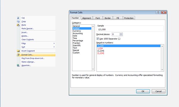
The same process can be accomplishing starting with a right click in the cell. Selecting the Format Cells option from the drop down menu will cause a dialog box to be displayed. Within this box are a number of options for formatting the cell and its contents.
After you've entered data, you may find that you need another column to hold additional information. For example, you may want to calculate the ratio of Total Cost Value to Sale Price and display the results in a column next to the Total Cost Value.
Or maybe you need another row, or rows. You might discover another sale parcel that you want to include in your analysis. That's great, but do you have to start over? Of course not.
To insert a single column, click any cell in the column immediately to the right of where you want the new column to go. So if you want a Ratio column between columns I and J, you'd click a cell in column J, to the right of the new location. Then, on the Home tab, in the Cells group, click the arrow on Insert. On the drop-down menu, click Insert Sheet Columns. A new blank column is inserted.
To insert a single row, click any cell in the row immediately below where you want the new row to go. For example, to insert a new row between row 4 and row 5, click a cell in row 5. Then in the Cells group, click the arrow on Insert. On the drop-down menu, click Insert Sheet Rows. A new blank row is inserted.
Excel gives a new column or row the heading its place requires, and changes the headings of later columns and rows.